Spike Synchrony
Contents
Spike Synchrony#
Neural synchronization can facilitate information transfer and the binding of information. Many methods have been employed to quantify nerual synchrony, and no one technique has become widely viewed as the gold-standard. Here, I will illustrate several methods to quantify neural synchrony, specifically:
Cross correlation
Unitary event analysis
Spike-triggered population rate
import elephant
import quantities as pq
from neo.core import AnalogSignal
from neo import SpikeTrain
import numpy as np
import matplotlib.pyplot as plt
import quantities as pq
import random
import viziphant.unitary_event_analysis as vue
from scipy.stats import norm, binom
from seaborn import color_palette
First, let’s simulate 2 neurons, synchronized to the same underlying oscillation (and consequently, synchronized to each other). Here, we can model this by generating two spike trains from the same underlying rhythmic firing rate.
np.random.seed(1224)
fs = 1000
times = np.arange(0, 2, 1/fs)
freq = 20
mean_rate = 60
osc = np.sin(2 * np.pi * times[:] * freq)
osc_rate = mean_rate * osc
osc_rate += mean_rate #make sure rate is always positive
sim_spike_rate = AnalogSignal(np.expand_dims(osc_rate, 1), units='Hz', sampling_rate=1000*pq.Hz)
st1 = elephant.spike_train_generation.inhomogeneous_poisson_process(rate=sim_spike_rate, refractory_period=3*pq.ms)
st2 = elephant.spike_train_generation.inhomogeneous_poisson_process(rate=sim_spike_rate, refractory_period=3*pq.ms)
Cross correlation#
Generating a cross correleogram is a good first step for assessing possible synchrony between neurons. A cross correlelogram shows the approximate timescale of this synchrony, as well as the rhythm that gives rise to the synchrony. Additionally, a cross correlation is relatively straightforward and common to compute. For more details, see the section on autocorrelation in spiketrain_analyses. This is the same analysis, but instead of comparing a spike train with itself, here we’re comparing two spike trains.
spikes1 = np.squeeze(st1)
spikes2 = np.squeeze(st2)

binsize = .005
max_lag = .1
start_win, stop_win = times[0] + max_lag, times[-1] - max_lag
histo_bins = int((max_lag*2)/binsize)

spike_diffs = []

for i, spike1 in enumerate(spikes1):
    if spike1>start_win and spike1<stop_win:
        for j, spike2 in enumerate(spikes2):
                spike_diff = spike1 - spike2
                if np.abs(spike_diff)<max_lag:
                    spike_diffs.append(spike1 - spike2)

plt.figure(figsize=(8,5))
counts, bins, patches = plt.hist(spike_diffs, bins=histo_bins)
plt.xlabel('Time lag (s)')
plt.ylabel('Count')
Text(0, 0.5, 'Count')
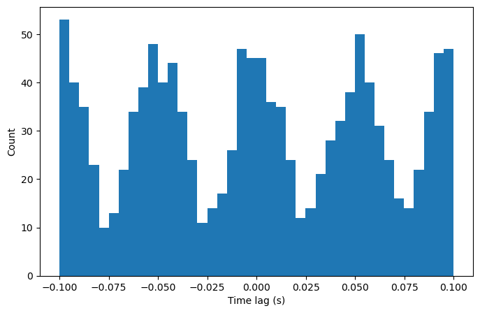
The bin at time lag = 0 can be used to assess synchronization. Here, the spike count at 0 is greater than the overall mean, suggesting these neurons are synchronous.
Unitary event analysis#
Unitary event analysis essentially computes the number of synchronous spikes [1]. Because some number of synchronous spikes are expected by chance, this number is then compared to an ‘expected’ number of spikes.
# Compute number of synchronous spikes
binned_st1 = elephant.conversion.BinnedSpikeTrain(st1, bin_size=5*pq.ms) #Binarize spike train
binned_st2 = elephant.conversion.BinnedSpikeTrain(st2, bin_size=5*pq.ms) #Binarize spike train

sync_events = np.logical_and(binned_st1.to_bool_array(),binned_st2.to_bool_array()) #Find where spikes occurred in both spiketrains
n_events = np.sum(sync_events)
n_bins = sync_events.shape[1]
print('Number of bins: '+ str(n_bins))
print('Number of synchronous events: ' + str(n_events))
Number of bins: 400
Number of synchronous events: 43
Now, let’s compare this number with how much we would expect by chance. There are a few ways to compute this. Analytically, we have two spike trains with a mean rate of 60Hz. Therefore, each neuron spikes .3 times per 5ms, and for any 5ms bin, the probability of both neurons spiking is .09. We can calculate the probability that we observe 43 synchronous events or greater using a binomial distribution.
# Analytic
p = binom.sf(n_events, n_bins, .09)
print('Analytic probability: '+ str(p))
Analytic probability: 0.09754615335115961
Though simple and efficient, this method works only when the firing rate of neurons is stationary over time. However, the firing rate of neurons can change over time, in ways that are correlated with one another that may be spurious to this analysis. This can occur with the onset of a stimulus, or a neuromodulator.
To deal with non-stationarities, there are several methods to create surrogate spike trains, which the actual number of synchronous events can be compared with [2]. Surrogates are commonly created by dithering (or jittering) a spike train by randomly moving each spike by some time within some small time frame. Alternatively, surrogates can be created by randomly shifting spike trains against each other, conserving the original structure of each spike train but requiring ultimately large time shifts. Finally, when analyzing synchrony evoked by a stimulus, spike trains can be shifted across trials, such that the number of synchronous events can be compared with the number of synchronous events found when comparing neurons recorded in different trials. However, this analysis assumes stationarity can be assumed across trials, which is generally unlikely.
Here, let’s dither to create surrogate spike trains, and compare the actual number of synchronous events with this distribution.
# Compare with surrogate spike trains
np.random.seed(2022)
surr_evts = []
surr_sts = elephant.spike_train_surrogates.dither_spikes(st2, 10*pq.ms, n_surrogates=200)
for surr_st in surr_sts:
    binned_surr_st = elephant.conversion.BinnedSpikeTrain(surr_st, bin_size=5*pq.ms) #Binarize spike train
    sync_events = np.logical_and(binned_st1.to_bool_array(),binned_surr_st.to_bool_array()) #Find where spikes occurred in both spiketrains
    surr_evts.append(np.sum(sync_events))
C:\Users\Michael\anaconda3\envs\tutorials\lib\site-packages\quantities\quantity.py:337: VisibleDeprecationWarning: Creating an ndarray from ragged nested sequences (which is a list-or-tuple of lists-or-tuples-or ndarrays with different lengths or shapes) is deprecated. If you meant to do this, you must specify 'dtype=object' when creating the ndarray.
  return np.multiply(other, self)
plt.hist(surr_evts)
plt.axvline(n_events, color='red')
plt.xlabel('# synchronous events')
plt.ylabel('Count')
plt.text(n_events+1, 30, 'Actual # events', color='red')

z_score = (n_events - np.mean(surr_evts)) / np.std(surr_evts)

dith_p = norm.sf(z_score)
print('Dithered probability: '+ str(dith_p))
Dithered probability: 0.10832211715896994
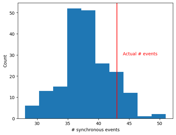
Now, let’s simulate two spike trains that only become synchronous after 1s.
np.random.seed(2022)
fs = 1000
times = np.arange(0, 2, 1/fs)
freq = 20
mean_rate = 60
osc = np.sin(2 * np.pi * times[:] * freq)
osc_rate = np.zeros(len(times))
osc_rate[1000:] = mean_rate * osc[:1000]
osc_rate += mean_rate #make sure rate is always positive
sim_spike_rate = AnalogSignal(np.expand_dims(osc_rate, 1), units='Hz', sampling_rate=1000*pq.Hz)
st1 = elephant.spike_train_generation.inhomogeneous_poisson_process(rate=sim_spike_rate, refractory_period=3*pq.ms)
st2 = elephant.spike_train_generation.inhomogeneous_poisson_process(rate=sim_spike_rate, refractory_period=3*pq.ms)
We can calculate how synchrony changes over time using elephant’s jointJ_window_analysis function, and plot it using the plot_ue function from viziphant (elephant’s companion visualization package).
spiketrains = [[st1, st2]]
random.seed(2022)
UEs = elephant.unitary_event_analysis.jointJ_window_analysis(spiketrains, bin_size=5*pq.ms, winsize=500*pq.ms, winstep=50*pq.ms, pattern_hash=[3])
vue.plot_ue(spiketrains, UEs, significance_level=0.05)
FigureUE(axes_spike_events=<AxesSubplot: title={'center': 'Spike Events'}, ylabel='Trial'>, axes_spike_rates=<AxesSubplot: title={'center': 'Spike Rates'}, ylabel='Hz'>, axes_coincident_events=<AxesSubplot: title={'center': 'Coincident Events'}, ylabel='Trial'>, axes_coincidence_rates=<AxesSubplot: title={'center': 'Coincidence Rates'}, ylabel='Hz'>, axes_significance=<AxesSubplot: title={'center': 'Statistical Significance'}>, axes_unitary_events=<AxesSubplot: title={'center': 'Unitary Events'}, xlabel='Time (ms)', ylabel='Trial'>)
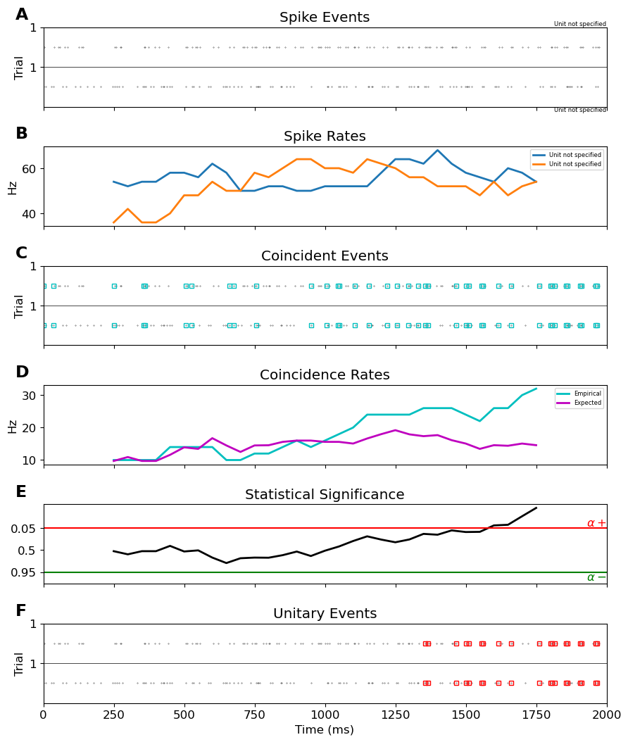
Elephant’s visualization shows many coincident events. Additionally, the actual coincidence rate is generally higher than the expected, as calculated analytically. However, the windows only reach significance around 1s, and only coincident events in these windows are marked as unitary events.
Spike-triggered population rate#
Alternatively, spike-spike synchrony can be computed as the spike-triggered population rate (stPR), or the firing rate of other neurons when one neuron fires [3]. This method has several advantages. First, the method can be used to test the synchrony between one neuron and a population of neurons. Therefore, when analyzing the general synchrony of each neuron, rather than neuron synchrony between individual neurons, this method can be much more efficient. Additionally, as demonstrated later, this method does not require the generation of surrogate neural spiketrains to control for a non-stationary spikerate. As a result, this method can be much more computationally efficient in analyzing the neural synchrony between a neuron and a population of neurons. Finally, this method provides a synchrony value for each spike, rather than for a given window of time, allowing for finer time resolution in analyzing synchrony.
To illustrate this method, we’ll start off by simulating a neuron, and a neural population, each firing in a synchronized rhythm.
#Simulate a neuron, and a neural population
np.random.seed(2022)
fs = 1000
times = np.arange(0, 2, 1/fs)
freq = 50
mean_rate = 60
osc = np.sin(2 * np.pi * times[:] * freq)
osc_rate = mean_rate * osc
osc_rate += mean_rate #make sure rate is always positiv
sim_spike_rate = AnalogSignal(np.expand_dims(osc_rate, 1), units='Hz', sampling_rate=1000*pq.Hz)
st2 = elephant.spike_train_generation.inhomogeneous_poisson_process(rate=sim_spike_rate, refractory_period=3*pq.ms)

n_pop_neurons = 10
st_pop = np.empty((0))
for n in range(0, n_pop_neurons):
    st = elephant.spike_train_generation.inhomogeneous_poisson_process(rate=sim_spike_rate, refractory_period=3*pq.ms)
    st = np.asarray(st)
    st_pop = np.concatenate((st_pop, np.squeeze(st)))

st_pop = SpikeTrain(np.squeeze(st_pop), units=pq.s, t_start=0 * pq.s, t_stop=(2 * pq.s))
Then, calculate the stPR, the mean firing rate of the population when neuron 2 fires.
#Calculate stPR (uncorrected)
spike_sr = 1000
sigma=5*pq.ms
kernel = elephant.kernels.GaussianKernel(sigma=sigma)
rate = elephant.statistics.instantaneous_rate(st_pop, sampling_period=1/spike_sr * pq.s,
                                              kernel=kernel, center_kernel=True)
rate = rate / n_pop_neurons
stPRs = []
spikes2 = np.squeeze(st2)
for spike in spikes2:
    stPRs.append(float(rate[int(round(spike * spike_sr, 4))]))

mean_stPR = np.mean(stPRs)
print('Mean firing rate: ' + str(np.mean(rate)))
print('Mean stPR: ' + str(mean_stPR*pq.Hz))
Mean firing rate: 59.576873252977244 Hz
Mean stPR: 66.67997370011862 Hz
The spike-triggered firing rate is greater than the overall mean firing rate, meaning neuron 2 is more likely to fire around when neurons in the population are firing relatively more.
Additionally, for each spike, we can get the firing rate in a surrounding window of time. This will allow us to see at what timescale the firing rate of neuron 1 increases when neuron 2 fires.
spike_sr = 1000
window = 100
sigma=5*pq.ms
kernel = elephant.kernels.GaussianKernel(sigma=sigma)
rate = elephant.statistics.instantaneous_rate(st_pop, sampling_period=1/spike_sr * pq.s,
                                              kernel=kernel, center_kernel=True)
rate = rate / n_pop_neurons
rate = np.asarray(rate)
stPR_segs = []
spikes2 = np.squeeze(st2)
for spike in spikes2:
    spike = float(spike)
    if spike > window/spike_sr and times[-1] - spike > window/spike_sr: #If window entirely within times analyzed
        rate_seg = rate[int(round(spike*spike_sr))-int(window/2):int(round(spike*spike_sr))+int(window/2)]
        stPR_segs.append(rate_seg)

stPRs_arr = np.asarray(stPR_segs)
stPRs_arr = np.squeeze(stPRs_arr)

plt.plot(np.arange(-window/2, window/2, 1), np.mean(stPRs_arr,0))
plt.xlabel('Time lag (ms)')
plt.ylabel('Population firing rate (Hz)')
Text(0, 0.5, 'Population firing rate (Hz)')
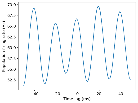
We have essentially created a cross correlation figure, using the firing rate of unit 1.
Controlling for firing rate#
However, this method is biased by the mean firing rate of the population: if neurons fire more in general, the stPR will be higher. Thus, just as with unitary event analysis, we need to find a method to control for the overall firing rate of the population.
In the original paper for this method, the authors did so via a shuffling method. Though their exact method does not suit our data, we can implement something similar by comparing with surrogate spike trains as we did before.
#Surrogate vs. real stPR
np.random.seed(2022)
surr_stPRs = []
surr_sts = elephant.spike_train_surrogates.dither_spikes(st2, 10*pq.ms, n_surrogates=200)
for surr_st in surr_sts:
    stPRs = []
    surr_spikes = np.squeeze(surr_st)
    for spike in surr_spikes:
        stPRs.append(float(rate[int(round(spike * spike_sr, 4))]))
    surr_stPRs.append(np.mean(stPRs))

plt.hist(surr_stPRs)
plt.axvline(mean_stPR, color='red')
plt.xlabel('stPR')
plt.ylabel('Count')
plt.text(mean_stPR+1, 30, 'Actual stPR', color='red')

z_score = (mean_stPR - np.mean(surr_stPRs)) / np.std(surr_stPRs)

dith_p = norm.sf(z_score)
print('Dithered probability: '+ str(dith_p))
Dithered probability: 3.5099805001481054e-08
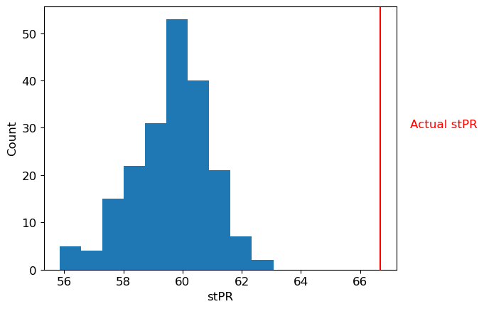
Alternatively, we can control for the overall firing rate of the population (and its nonstationarities) in our measurement of the firing rate itself. We can isolate the fine-timescale deviations from the mean firing rate by substracting out the longer-timescale estimate of firing rate. Specifically, this method measures firing rate on a fine time-scale using a narrow kernel, and subtracts the firing rate measured on a slow timescale from this firing rate.
First, let’s isolate the fine-timescale fluctuations of the population by substracting out a longer-timescale estimate of firing rate. We’ll add a simulation of a slow fluctuation in firing rate, to illustrate how we can remove it with this analysis.
#Isolate fine-timescale firing rate fluctuations
fast_kernel_sigma = 3*pq.ms
slow_kernel_sigma = 11*pq.ms
fastk = elephant.kernels.GaussianKernel(sigma=fast_kernel_sigma)
slowk = elephant.kernels.GaussianKernel(sigma=slow_kernel_sigma)

fast_rate = np.asarray(elephant.statistics.instantaneous_rate(st_pop, sampling_period=1/spike_sr * pq.s,
                                                       kernel=fastk, center_kernel=True))
slow_rate = np.asarray(elephant.statistics.instantaneous_rate(st_pop, sampling_period=1/spike_sr * pq.s,
                                                       kernel=slowk, center_kernel=True))
fast_rate /= n_pop_neurons
slow_rate /= n_pop_neurons
fast_rate = np.squeeze(fast_rate)
slow_rate = np.squeeze(slow_rate)
freq=1
osc = np.sin(2 * np.pi * times[:] * freq)
fast_rate += np.squeeze(osc*20) #Add general drift to the firing rates
slow_rate += np.squeeze(osc*20) #Add general drift to the firing rates
diff_rate = fast_rate - slow_rate
colors = color_palette("flare")
plt.figure(figsize=(11.5, 8))
plt.subplot(2,1,1)
plt.plot(times, fast_rate, color=colors[3], label='fast rate')
plt.plot(times, slow_rate, color=colors[-1], label='slow rate')
plt.legend()
plt.subplot(2,1,2)
plt.plot(times, diff_rate)
plt.legend(['fast - slow'])
plt.xlabel('Time (s)')
plt.ylabel('Firing rate (Hz)')
Text(0, 0.5, 'Firing rate (Hz)')
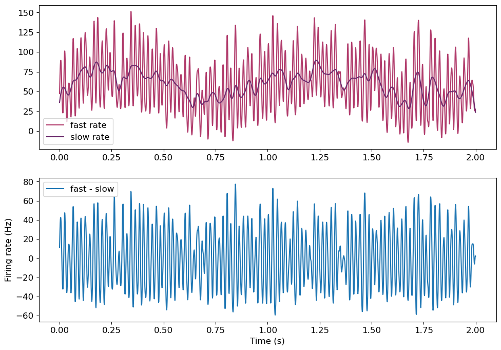
The fine-timescale kernel firing rate tracks the high frequency oscillation, while the slow-timescale kernel does not. Still, the slow kernel tracks the non-stationary firing rate. Substracting this from the fast kernel removes the slower drift in our data. Now, firing rate has a mean of 0, and positive values indicate a relative increase in firing rate, while negative values indicate the reverse. Now, we can calculate the stPR on this difference.
stPRs = []
spikes2 = np.squeeze(st2)
for spike in spikes2:
    stPRs.append(float(diff_rate[int(round(spike * spike_sr, 4))]))

mean_stPR = np.mean(stPRs)
print('Mean firing rate: ' + str(np.mean(diff_rate)*pq.Hz))
print('Mean stPR: ' + str(mean_stPR*pq.Hz))
Mean firing rate: 0.18442787923700246 Hz
Mean stPR: 16.170752011037074 Hz
The stPR is much higher than 0, indicating the neuron is synchronous with the population. Notably, unlike the other methods, this analysis does not provide a significance value. Still, these values can be compared between neurons, or with a baseline.
Kernel Design
We can get a more exact idea of what firing rate changes this timescale is estimating by plotting how each kernel estimates the firing rate of a single spike.
#Kernel design
fast_kernel_sigma = 3*pq.ms
slow_kernel_sigma = 11*pq.ms
spiketrain = SpikeTrain([-1, 0, 1], t_start=-1, t_stop=1, units='s')
time_array = np.linspace(-50, 50, num=1001) * pq.ms
kernel = elephant.kernels.GaussianKernel(sigma=fast_kernel_sigma)
fast_kernel_time = kernel(time_array)
kernel = elephant.kernels.GaussianKernel(sigma=slow_kernel_sigma)
slow_kernel_time = kernel(time_array)


colors = color_palette("flare")
plt.figure(figsize=(11.5, 4))
plt.subplot(1,2,1)
plt.plot(time_array, fast_kernel_time, color=colors[3])
plt.plot(time_array, slow_kernel_time, color=colors[-1])
plt.legend([str(fast_kernel_sigma)+' kernel', str(slow_kernel_sigma)+' kernel', 'Difference'])
plt.xlabel("time, ms")
plt.ylabel("kernel, 1/ms")
plt.xticks([-25, -5, 5, 25])
plt.axvline(-5, color='black', alpha=.4)
plt.axvline(5, color='black', alpha=.4)
plt.xlim(-30, 30)

plt.subplot(1,2,2)
plt.plot(time_array, fast_kernel_time-slow_kernel_time, color=colors[2])
plt.xlabel("time, ms")
plt.ylabel("kernel, 1/ms")
plt.axvline(-5, color='black', alpha=.2)
plt.axvline(5, color='black', alpha=.2)
plt.axhline(0, color='black', alpha=.2)
plt.xticks([-25, -5, 5, 25])
plt.xlim(-30, 30)
plt.legend(['Difference'])
<matplotlib.legend.Legend at 0x21f5ffc3850>
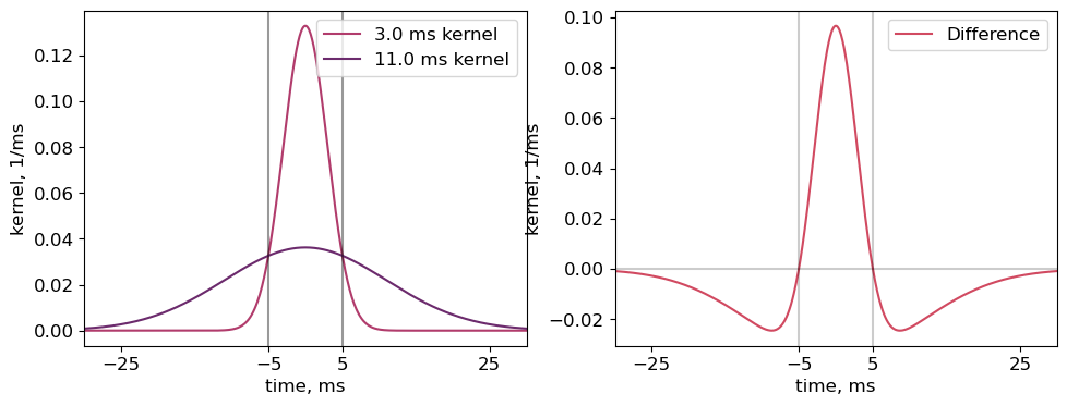
The narrower kernel results in an estimatation of firing rate that only increases immediately surrounding the spike, but increases to a much higher degree. Specifically, using a 3ms and 11ms sigma for the fine and slow time-scale kernels, respectively, the fine-timescale firing rate is increased in the 10ms surrounding the spike, but decreased in the remaining 60ms. Therefore, this metric will be positive when the difference between two spike times is less than 5ms, or negative when the difference is between 5 and ~30ms.
Using this method, the timescales of the kernels should be carefully designed to reflect what the study would like to define as synchrony, and what general fluctuations should be removed.
Convolution of a cross correlation#
Other studies have convolved the cross correlation histogram, rather than the spike trains themselves, to estimate synchrony. Specifically, after a cross correlelogram has been computed, slower covariations in firing rate are estimated by convolving the cross correlelogram with a gaussian kerenel. The significance of each bin can then be compared to the convolved correlelogram, asssuming a poisson distribution [4]. This method therefore allows for the estimation of significance without jittering. Additionally, this method can also be applied towards identifying peaks in the cross correlelogram at time lags other than 0, for example, to identify a monosynaptic connection between neurons from a peak at +3ms [5]. However, the time resolution of this method is limited, as a cross correlelogram must be computed with a sufficent time window to include a reasonable estimate of the distribution at various time lags. This method has not been used by our lab, but the Buzsaki lab has published example code on Github.
References#
Grün, S., Diesmann, M., Grammont, F., Riehle, A., & Aertsen, A. (1999). Detecting unitary events without discretization of time. Journal of neuroscience methods, 94(1), 67-79
Grün, S. (2009). Data-driven significance estimation for precise spike correlation. Journal of Neurophysiology, 101(3), 1126–1140. https://doi.org/10.1152/jn.00093.2008G
Okun, M., Steinmetz, N. A., Cossell, L., Iacaruso, M. F., Ko, H., Barthó, P., Moore, T., Hofer, S. B., Mrsic-Flogel, T. D., Carandini, M., & Harris, K. D. (2015). Diverse coupling of neurons to populations in sensory cortex. Nature, 521(7553), 511. https://doi.org/10.1038/NATURE14273
Stark, E., & Abeles, M. (2009). Unbiased estimation of precise temporal correlations between spike trains. Journal of Neuroscience Methods, 179(1), 90–100. https://doi.org/10.1016/J.JNEUMETH.2008.12.029
English, D. F., McKenzie, S., Evans, T., Kim, K., Yoon, E., & Buzsáki, G. (2017). Pyramidal cell-interneuron circuit architecture and dynamics in hippocampal networks. Neuron, 96(2), 505. https://doi.org/10.1016/J.NEURON.2017.09.033

